Participation Assignment #2

The article that I found is an interesting application to GIS. This describes how, in 1996, TransCanada used GIS to select the best route for an expansion pipeline. I found it interesting because this seems to be one of the first times this type of analysis took place using GIS. It's a route selection analysis very similar to what we did early in the semester in the other course with the corridor analysis. They set the project goals, which were threefold. First, minimize risk to public safety. Second, minimize environmental impact. Third, minimize construction and operation costs.

This particular project used information from already existing digital and map sources and interpreted imagery. They used GIS techniques to include “exclusions, constraints, and opportunities.” When minimizing environmental impacts, they weighted environmentally sensitive areas with heavier constraints. Collocations with already existing rights-of-way were weighted with lower constraints, so the GIS could label them as opportunities. They also weighted river and road crossings heavier, as that would increase construction costs. They also created buffers around urban areas to minimize the impact on the population.

Using these criteria, TransCanada developed several route alternatives. The GIS was able to provide the lengths of the routes and detailed crossings information. They also analyzed the impacts of the different criteria on the various alternative routes. Before selecting a preferred route, more data were gathered based on aerial imagery and ground-truthing. This method became a go to method for other entities for route selection, and it is very similar to scenarios we have seen in the other course.

GIS-based process helps TransCanada select best route for expansion line

Module 10 - Creating Custom Tools

In this assignment, we learned to create custom tools and toolboxes. First, we were create a script tool from a provided script, which was to run in ArcMap. I opened the script and modified the script name, last modified date, and modified by comments, and saved it under my name. In ArcMap (ArcToolbox) I created a new toolbox, and within that toolbox, a new script. Creating a new toolbox was rather straightforward, was just right-click -> New Toolbox; very similar to making a new folder. Next we were to set parameters. Creating the parameters is pretty simple tool, as in Properties there is a tool dialog box that makes it easy to not only create parameters, but to modify their settings (data type, multivalue property, etc.). Below is a screenshot of my script tool window.

Now that the parameters are set in the script tool, they needed to be set in the script. I changed the original four variables in the script, replacing them with the arcpy.GetParameter() command. I had a little bit of an issue here, as I was using the arcpy.GetParameterAsText() command initially. This didn’t work, as this only reads parameters as text, which caused errors. As the outputFolder can’t be concatenated with strings, I used the str() function on the outputFolder variable, and ran the tool. Next we were to replace the print statements with arcpy.AddMessage() statements. Initially, I did this and no matter what I did, I could not get the code to work when running it. The problem turned out not to be in the code. What was going on is that I was trying to run the script in PythonWin as a stand-alone script. The arcpy.AddMessage() statements are, I think, designed to be run as a script tool. When I opened ArcMap and ran the tool again, it worked fine. Below is a screenshot of my results window.

To share the toolbox, tool, and script, I selected both the toolbox and the script and sent them to a compressed (zipped) folder.

I feel I learned a lot in this lab, and I think I’ll get a lot of use out of using toolboxes and tools in the future. I think one of the most valuable components of this lab is the idea of sharing the tools and toolboxes. Once I figured out the couple of issues I had and why what I was doing was causing problems, the assignment seemed pretty straightforward. Creating toolboxes is rather user-friendly and should be picked up quickly by most people familiar with Windows. The same can be said for setting the parameters in the dialog box, although it’s important to get the settings such as “Multivalue” correct, or the tool won’t run properly; it is easy to go back and check those, though. Once I understood what the arcpy.GetParameter() and arcpy.AddMessage() functions are doing, I realize they are quite useful and I’ll try to find ways to use them in the future. I also like the idea of sharing toolboxes and scripts, so others can use or modify them.

Module 9 - Working with Rasters

This assignment taught us to work with rasters using Python. We worked with 2 rasters, elevation and landcover, to create a Python script is a single raster image with the following criteria: 1) Forest landcover classification; 2) slope between 5 and 20 degrees; and 3) aspect between 150 and 270 degrees.

It is becoming almost habit to start off by importing the necessary modules needed for the script and to set the overwrite output to true. For this assignment, I attempted to create the output in a .tif format, but I got several errors, so I went with the optional part and created a file geodatabase. For the rest of the script, the module exercise was extremely helpful and relevant to the assignment. I created a conditional statement so the script would only run if the Spatial Analyst extension was available. Further down toward the end of the script, there is an else statement printing a message if it is not available. Within the if statement is where the bulk of the script is located, as I only want it to run if the spatial analyst module is available. I used the remap value and reclassify tools to reclassify the landcover raster so that only the forested areas are given a value of "1". I assigned the elevation raster to a variable and used the slope and aspect functions to create temporary rasters of those types. I was impressed with how user friendly the map algebra commands are when used in Python, so performing the slope and aspect calculations weren't an issue. I created temporary rasters based on the 3 criteria listed above and using "less than" and greater than" statements in the script. I combined the 5 rasters (four slope and aspect rasters and the reclassified landcover raster), and saved it to make it a permanent raster. Below is a screenshot of the raster, with the "0" (reddish-brown in color) signifying areas of the landcover raster not classified as forest and areas labeled as "1" (the green areas) showing areas that are forest land cover.

This assignment was far less stressful for me than last week's assignment. I feel I have a greater understanding of this concept, and the exercise was extremely helpful, so if I had a syntax error I could look at the exercise (and the textbook) to determine if I was missing a parentheses or whatever the error was. The only issue I had dealt with the file geodatabase I created. Even setting the overwrite output to true does not allow you to overwrite the geodatabase, which I suppose makes sense. The geodatabase has files within it, and you usually can't overwrite a non-empty folder. I was unable to find any workaround, so after running the program once, you still have to go into the Results folder and delete the geodatabase. I didn't do this as it just occurred to me while writing this, but I wonder if it's possible to have the code delete the files within the geodatabase at the end of the script, and then have Python overwrite the empty geodatabase. I liked working with rasters in this assignment and I was impressed that Python almost seems to be made to work with some of the map algebra operators. I like that a relatively short and simple code can do this much geoprocessing. On another note, the ELearning site appears to be down, so I chose to email the instructor the relevant deliverables.

Module 8 - Working with Geometries

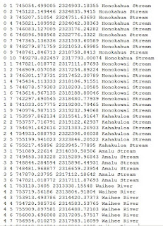
This week’s lab dealt with working with geometries in Python, and it was a challenging one for me, partially because working with arrays and nested loops are not my strong suit and partly due to a pretty intense work schedule this week. In this lab, we were working with the “rivers.shp” file, using loops to iterate through the cursor, and we wrote the data to a .txt file.

After importing the modules and setting the workspace, I created a search cursor for the shapefile I was working with. This called the OID field, the SHAPE geometry object, and the NAME field. I created a .txt file using the write mode, following examples in the text and in our exercise. To write the data to a text file, I needed to create a couple of “for” loops. The first iterates through each row in the shapefile’s attribute table. I created a variable called vertexid within the loop set to 0, so that it resets for each new feature. Within that loop, I created a second loop using the .getPart() method, which iterates through each point in the array of the row. The .getPart() method allows me to access the points in each array. If I did not use this method, another “for” loop would be necessary. I added “1” to the vertexid variable in this loop to keep track of the number of points in each feature.

Here’s where it got tricky for me. I needed to use the write() method to write to the .txt file. I wanted to add the Feature/row ID, the vertex ID, the X and Y coordinates, and the name of the river feature, using “\n” to ensure each vertex is on its own line. I ran into a wall here with syntax errors and exceptions at first. I was pretty sure the loops were correct (at least mostly) because I immediately was able to print correct values for the X and Y coordinates. I ran into a syntax error which gave no input into where or what the error was, so I started deleting code (remembering later I could have commented it out) and attempted to run the program. The issue turned out to be a print statement I had created underneath the write() statement, which wasn’t necessary, so I just left it out. The other error I had was not using arrays properly. I had the output in the .txt file correct, but the name and feature were printing “NAME” and “FEATURE”. Once I changed this to row[2] in the write() statement, the program wrote to the .txt file correctly. The output is shown below.  The first column shows the Feature/row ID, the second column shows the vertex ID for that feature (notice how it resets for each feature), the 3^rd and 4^th columns are the X and Y coordinates of the vertex, and the 5^th and 6^th columns are the feature name and type.

This was a really good lab, as I learned about working with geometries and got more experience working with arrays. Both the instructor and the other students on the discussion boards were a big help with steering me in the right direction with my code. I wish I had had more time to really work with it, as opposed to an hour or two at a time, but even so, I learned a lot and I think it’s less confusing and less intimidating to work with than with FORTRAN or even IDL code.

Lab 8 - Damage Assessment

In this lab, we carried out a building damage assessment based on aerial imagery taken before and after Superstorm Sandy impacted the northeastern United States. Although not especially powerful as far as some hurricanes can be, the extreme size of the storm, the fact that it collided with a powerful weather system moving into the northeast, and its impact on several of the U.S.’s largest cities (including a historic storm surge), combined to make it the second costliest cyclone to hit the United States since 1900.

First I created a base map using the World Countries, US boundary, and FEMA States shapefiles. The FEMA shapefile was created from a selection of impacted states from the US boundary shapefile. After importing the Sandy storm track table, I created a polyline showing the storm’s path from the original hurricane track points. I learned to create marker symbols, and symbolized the hurricane with a hurricane symbol. I used a color scheme from green to red, with green showing where Sandy was less powerful and red at the storm’s most powerful, in this case a Category 2 hurricane. I labeled the hurricane track points and added graticules and the essential map features. Below is my final map.

Next I needed to prepare the data for the damage assessment. This was achieved by creating a new file geodatabase and new raster mosaics, one for the pre-storm imagery and one for the post-storm imagery. I briefly learned to compare the before and after imagery by learning the Flicker and Swipe tools in the Effects toolbar. One of the most important aspects of the assignment was creating attribute domains, which are used to constrain values allowed in an attribute table or feature class. Shown below is a screenshot of domains I created for the damage assessment. Damage ranges from 0 (no damage) to 4 (total destruction).

I added the county parcels and the study area layers to our map. This part was quite time consuming, as I had to digitize each structure from the pre-storm image within the study area, and then compare the pre-storm and post-storm imagery to determine the level of damage the structure received. This was often difficult to determine, as I was using aerial imagery and it was difficult to see much of the damage unless it was very severe. It was also often difficult to determine the building type (residential, commercial, or industrial).

Next I wanted to examine the relationship between the locations of the damaged structures and their proximity to the coastline. I digitized the coastline near the study area and used Select by Location to determine the number of damaged structures within 100 m, 100-200 m, and 200-300 m from the coastline. As one would imagine, structures closer to the coastline were more likely to be destroyed or suffer catastrophic damage, and those further from the coastline were more likely to suffer little to no damage. Structures blocked from the winds and/or water had a better chance of surviving intact as well. Below is a table of the structural damage.

                                                 Count of structures within distance categories from the coastline

Structural Damage Category
	0-100 m	100-200 m	200-300 m
No Damage	0	0	7
Affected	0	6	7
Minor Damage	0	26	22
Major Damage	2	6	2
Destroyed	10	10	4
Total	12	48	42

I used the Attribute Transfer tool to copy the attributes from the county parcels layer to the structure damage layer. To populate the new fields, I manually matched the parcel to the damaged structure point. Once I had done this for all the damage points, I exported the data to an Excel spreadsheet and labeled the points. The purpose of this was to help determine who owns the damaged structures for emergency management and insurance purposes.

This lab seems to cover most of what damage assessment is used for. Although manually digitizing is rather tedious, it helps determine the extent of the damage. In a real situation however, I would be more comfortable creating the initial assessment using aerial imagery, but actually going through the area to visually confirm the assessment values would be important as well.

Module 7 - Explore/Manipulate Spatial Data

In this assignment, we learned to explore and manipulate spatial data in Python. I found this to be a great introduction to manipulating spatial data and I learned how to use some functions that I had no experience with. The objective was to create a script that created a new geodatabase, copied data from the data folder into the new geodatabase, and populated a dictionary with the names and population of county seats in New Mexico.

First I imported the modules and set the environments so that the output could be overwritten. Then I created a new geodatabase and set my current workspace. I needed to create a variable returning a list of all feature classes in the workspace folder. I used a “for” loop to copy feature from the workspace to the new geodatabase. Here, I made a simple mistake that took a little bit to find. I inadvertently set the workspace and the new geodatabase to the same location, so I had to correct that. The new files use the basename property from the arcpy.Describe() function. I then created a search cursor for the cities layer. It took a while to get the syntax correct, and I tried some different options with delimiting the FEATURE field. This part of the lab was tricky with getting the single and double quotation marks correct. Then we started working with dictionaries. I created an empty dictionary, which I was to then populate. This step took me the longest, and the issue was mainly just figuring out the proper syntax to do what I wanted to do. I wanted the county seats and their populations, but I had to select the county seats from the cities field, which added some complexity to the script. I added print messages to each step and made sure to comment the script.

Looking back over the exercise for this assignment was a big help, as sometimes I couldn’t remember the syntax exactly or which command to use in my script. We were provided a template, which was helpful for the most part. It was helpful to see in which order we were to perform a step, but sometimes when the code for that step was only one line I wondered if I was missing something. I also have a comma in my dictionary instead of a colon separating the fields in the output; I’m not sure what’s causing that, but the code does work without error. Below is a screenshot of the output (no actual code).

Lab 7 - Coastal Flooding

In this assignment, we learned to use elevation models to analyze impacts of coastal flooding. In the first part, we used a high-res LIDAR DEM for Honolulu, Hawaii to determine the impacts of two sea-level rise scenarios. We examined the population impacted by the flooding and analyzed the population distribution impacted and how it differed (or didn’t) from the overall population. In the second part, we compared the use of two elevation models for Collier County, Florida to determine the extent of flooding due to a 1 meter storm surge, and analyze the differences between the two results.

In the first part, I wanted to assess the extent of the area of impact of flooding due to a 3 foot sea level rise and a 6 foot sea level rise. I used the Lidar DEM and the desired sea level rise value as inputs to create rasters showing flooded and non-flooded areas for both scenarios. After I created the rasters showing the flooded areas, I was able to calculate the area flooded for the two scenarios. As expected, the area flooded from a 6 ft sea level rise is much greater than that flooded by a 3 ft sea level rise. Next, I wanted to investigate sea level rise vs. population density in the 6 foot sea level rise scenario. Values were calculated with the Field Calculator. The map below shows 1) the flooded area for the 6 ft scenario, 2) the flooded depth within the flooded area, and 3) the population density by census tract.

I then wanted to determine the population affected by the rise in sea level. For this I needed to convert the raster into a polygon and used the “centroid containment” analysis to include block groups whose centroids are within the flooded area. I added fields to the table and calculated the percent of various demographics that are affected by the flooding. From this, it can be seen that over 60,000 people are affected by flooding, although over 1.3 million are not flooded. As far as demographics are concerned, 35% of those affected are white, ~32% are owner occupied residences, and over 16% of those affected are 65 years of age or older. Of those not flooded, a quarter are white, over half are owner occupied residences, and ~13% are 65 years of age or older.

In the second part of the lab, I wanted to determine the impact of a uniform 1 meter storm surge on Collier County, Florida. Of course, storm surges are not usually uniform, but this is a good example of coastal flooding.  Using LIDAR and USGS elevation models, I wanted to show which cells are flooded. One catch here was that the LIDAR elevation model was in feet so I needed to convert from feet to meters. After creating rasters showing flood areas as an elevation less than 1 meter, there were a few disconnected areas; areas below 1 meter that were further inland and surrounded by higher elevation and won’t flood from a storm surge. Using the Region Group tool allowed me to eliminate those areas by only selecting regions connected to the coast, ensuring I was getting areas that will flood as they are directly connected to the incoming storm surge. I was able to determine how many buildings of which type were impacted and from that, compare the reliability of the elevation models in modeling coastal flooding due to a storm surge. When calculating the errors of omission for the LIDAR elevation model, I found that it was consistently undercounting the number of buildings by a little over 30% overall. The USGS model seemed to be a little more reliable, overcounting the number of buildings that would be flooded by about 8% overall.

I learned a lot about comparing the two elevation models and how the results can differ depending on which you choose to use. I still need some practice with calculating errors of omission and commission, but the concept makes sense. Of course, storm surges are not a uniform height. One needs to take into account the strength and speed of the storm causing the storm surge, the size of the coastline, whether there are any coastline features that help inhibit or enhance the storm surge, etc. That being said, I did enjoy this lab and learned a lot about modeling coastal flooding using GIS.