Lab 8 - Thermal and Multispectral Analysis

       In this lab, we learn to interpret radiant energy, to create composite multispectral imagery in both ERDAS Imagine and ArcMap. We also learn to change band combinations, and we further investigate adjusting imagery by adjusting breakpoints.

   This exercise demonstrates the basic principles of thermal energy and radiative properties, specifically the concepts associated with Wien’s Law and the Stefan-Boltzmann Law. The radiant energy is proportional to the fourth power of an object’s temperature, so the Sun emits more radiant energy than the Earth. We also see that the energy peak moves to shorter wavelengths as the temperature increases. This is why we call incoming solar radiation “shortwave” radiation and outgoing terrestrial radiation as “longwave” radiation.

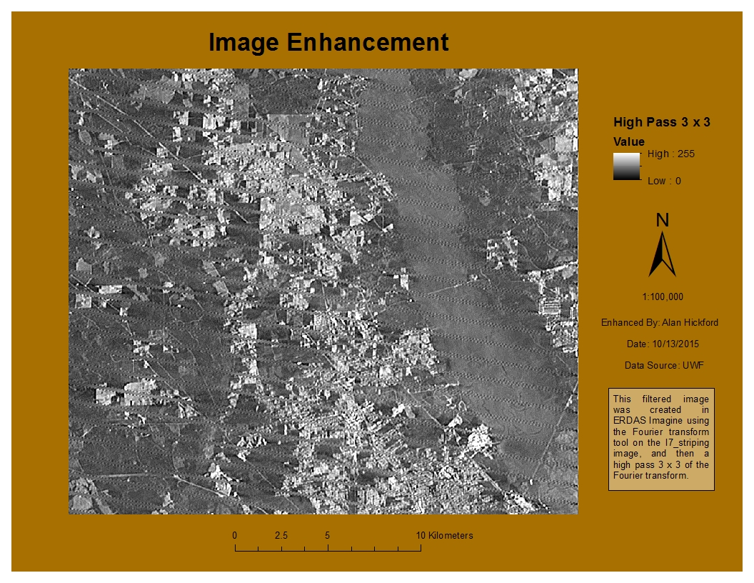
.      The second exercise of the lab is a really good introduction to combining multiple layers into a single image file both by using Layer Stack in ERDAS and Composite Bands in Arcmap. As pointed out in the lab, it is much quicker and easier in Arcmap, but it’s good to know how to do this in ERDAS as well.

.      We also learned to analyze the image, both in panchromatic and multispectral bands, and manipulated the different spectral bands being displayed by manipulating the breakpoints to better distinguish certain features. We saw the difference between images taken in winter versus images taken in summer by looking at the thermal infrared band. It’s really interesting to see the diurnal pattern and the differences in specific heat capacity, with features that heat up quickly during the day also cooling quickly at night or in winter.

       The final portion of the lab tasked us with displaying different bands of multispectral imagery I decided to use the Pensacola composite image and to identify urban features. I still am learning how to adjust breakpoints, but this part gave me a lot of practice with it. I also used a lot of trial and error regarding which bands of the imagery would best display the feature that I wanted, which was rather tricky. Often, the urban areas were not displayed well; they were usually too light and although you could see the general area, you couldn’t really distinguish any features. Using the bands I chose, there is good contrast between the urban areas and adjacent areas, such as the water and the vegetation, and the urban areas are pretty well defined. Below is my image of Pensacola. The feature I wanted to identify was the urban areas, and they are clearly defined as the pink/lavender area, mainly west of the river that runs north-south through the middle of the image. For this image, I am displayed bands 1, 4, and 6. Band 1 shows blue wavelengths, and is often used to display man-made features. Adjusting the breakpoints of this band made the image clearer. Band 4, or near-IR, is often used to identify vegetation, but here after adjusting breakpoints to limit the amount of red in the image, the urban areas stood out. The band that completes the image is band 6, which is thermal IR. Urban areas are often warmer than surrounding areas, and that is the case here. Additionally, with the thermal IR layer, you can clearly see the fire in the far northeast portion of the image.

       

     

Lab 9 - Accuracy of DEMs

The objective of this assignment was to calculate and analyze the vertical accuracy of a DEM, comparing it to known reference points. We also analyzed the effects of interpolation methods on DEM accuracy.

First, we are given a high resolution DEM obtained through LIDAR and reference elevation points collected on the ground. Field data was collected for 5 land cover types: a) bare earth and low grass, b) high grass, weeds, and crops, c) brush lands and low trees, d) fully forested, and e) urban areas. Cluster sampling was used, which are selected by a random or systematic method with a cluster of samples around each center. The main way to spot cluster sampling is that the distances between samples are smaller than the distance between clusters.

One of the best ways to determine the quality of a DEM is to take the DEM data and compare it to some form of reference data. Here we used elevation points obtained from the field. Using that data, we can determine the root mean square error (RMSE), the 68^th percentile accuracy and the 95^th percentile accuracy. Low values there generally means that the DEM data matches up well with the reference data and the values are accurate. You can also calculate the mean error to help determine the vertical bias. The reason RMSE does not work for this is that the elevation difference between the DEM and reference values are squared within the calculation, so the result is always positive; you cannot determine bias from RMSE. From my results, this is a very accurate DEM, with an overall RMSE of 0.276 meters and a 95% confidence level of 0.43 meters. It seems to be the most accurate over bare earth and low grass and less accurate over shrubland and low trees (perhaps it’s easier to distinguish between taller trees and the ground than shrubs and the ground). The vertical bias is also very small, with a combined vertical bias of 0.006 meters. The greatest vertical bias is a 0.16 m negative bias over urban areas and a positive 0.10 m bias over brush land and low trees. The LIDAR data seems to be an excellent model of elevation here, and it does exceptionally well over flatter (less “rough”) areas, such as bare earth or low grass.

Next we are provided a data layer contained 95% of the total points, which are used to create DEMs using 3 interpolation methods: IDW, Spline, and Kriging. The remaining 5% of the points are used as reference points. After creating the 3 DEMs, I exported the reference data to an Excel file and created new columns for the DEM data. After inputting the data to the Excel file, I performed the RMSE, 68th and 95th percentile, and mean error calculations for the three DEMs. Based on these calculations and assuming that I want the interpolation elevation values to be the closest to the reference points, the best interpolation technique for this particular data set is the IDW interpolation.

Statistic	IDW	Spline	Kriging
RMSE (m)	11.78366	17.78546	12.11856
95th	21.72756	20.04868	22.60116
68th	12.18899	9.888262	12.41265
ME (m)	1.73996	0.854330	2.121384

Overall, I learned a lot about the process of determining the vertical accuracy of DEMs using reference points. I initially had some difficulty figuring out how to determine the 68th and 95th percentile accuracies, but going back to a previous lab helped with that.

Lab 8 - Surface Interpolation

In this lab we learned to use ArcMap to carry out and interpret various surface interpolation techniques, including Thiessen, IDW, and Spline.
First, I used given elevation points with interpolation techniques to create a DEM using the Spatial Analyst toolbar in ArcMap. The two techniques used were the IDW method and the Tension Spline method. I wanted to see the differences between the two methods so I used the Raster Calculator to subtract the values of the DEM spline grid from those from the DEM IDW grid. The map layout is seen below.

The areas in the brightest red shows areas where the results of the IDW technique show an elevation nearly 40 m greater than those of the Spline method, and the brightest green shows where the Spline method is nearly 40 m greater than the results of the IDW method. When looking at the values of the elevation points, which are about 425 m, I can see that some of the differences between the results approach 10% of the total elevation, which definitely should affect the DEM.

In the second part of the lab, I wanted to use various spatial interpolation techniques to determine which worked best on water quality data for Tampa Bay. Technique 1 was a non-spatial technique, where I used the Statistics tool on the data points. Technique 2 is Thiessen interpolation, which assigns each location the same value as the nearest point.  In ArcMap I used the Create Thiessen polygons tool, converted it to a raster, and used the Zonal Statistics tool to determine spatial statistics.I wouldn't use this technique in this case as I'm pretty sure water quality in unsampled locations is not necessarily the same as at the sampled locations; the data is not that densely sampled. Technique 3 was IDW and technique 4 was spline interpolation. As IDW estimates cell values by averaging the values of sample points in the neighborhood of each processing cell, this method works better with densely sampled data, and seemed to work well with the water quality data. Spline interpolation minimizes overall curvature and results in a smooth surface passing through the sample points, and this worked fairly well for the water quality data once it was modified. The spline technique originally resulted in abnormally high maximas and minima with negative values. Much of this was due to some data points that were very close in proximity to each other had largely different values, which caused abnormally high and low extremes nearby. Once this data was modified, the spline interpolation worked well. As far as which interpolation technique, to me it would depend partially on if I knew whether or not the maximum and minimum values were included in my sample points. If I knew they were or if the data was densely sampled, I would go with IDW interpolation as it is an exact interpolator and will not result in values outside the sampled maximum and minimum. Spline interpolation is not an exact interpolator, so if I'm not sure the maximum and minimum have been sampled or if the data is not densely sampled, I would consider using spline interpolation.

Lab 6 - Image Enhancement

In this lab, we learned three main concepts. First, we learned to download and import satellite imagery into ERDAS Imagine and ArcMap. We also learned how to perform spatial enhancements using both of the mentioned software programs, and we learned to use Imagine to perform Fourier transformations.

First, we learned to obtain satellite imagery and how the files are named on the glovis.usgs.gov website. It’s pretty straightforward, with the names following a Sensor type, Path and Row number, and date in the form of year and the Julian date. Of course, other sources of data may have different methods of naming the data files.

         We also learned how to unzip these specific types of files, which are downloaded in a *.tar.gz format. I use this type of file quite often, and this is fairly simple to unzip, you just use the 7-Zip software on the file twice.

    The second part of the lab involved learning about different types of spatial enhancement in both Imagine and ArcGIS. I found this really interesting because it gave me a better understanding of what exactly occurs when you use a high or low pass filter. It's used a lot when performing research in meteorology, so I already had a basic understanding of it, but this lab explains it well and is very useful, especially seeing the calculations being performed when using the filters.

     We learned about high pass filters, which allow high frequency data (data that changes rapidly from pixel to pixel) to pass through, but suppresses low frequency date (data that doesn't change much from pixel to pixel). This has the effect of enhancing edges or discrete features, or to sharpen an image. We also learned about low pass filters, which allow low frequency data but suppress high frequency data, which has the effect of blurring or "smoothing" an image. I also learned how to use the Focal Statistics tool in ArcMap, specifically the "Mean" and "Range" filters. The Mean filter is a low pass filter, but it uses as 7x7 kernel instead of a 3x3 kernel, which results in each new cell being the average of a larger area, so the result is a more generalized image. I immediately thought in terms of resolution -- the results from the 7x7 kernel having a more coarse resolution than those from the 3x3 kernel. The Range statistic is similar to Edge Detect, It gives each new cell a value showing the difference in brightness between neighboring pixels, which is called spatial frequency. So, if you have a border or an edge, the spatial frequency will be high and it will show up brighter on imagery. The interiors of an area will be darker as they will have a lower spatial frequency due to the similarity of the surrounding pixels.

    

      The third part was the main focus of the lab. We were to take an image and perform an enhancement on it that reduced the effect of the striping in the image, but also retain most of the detail. I performed a Fourier transform on the image using Imagine, which reduced some of the striping. I then used a 3x3 Sharpen kernel on the image to sharpen the features. I really enjoyed working with the Fourier transform tool. I have seen it used in statistics and research, but never actually worked with it before (outside of mathematics). It wasn't too complicated to perform the transformation with Imagine, and I used it in my final enhancement image. I created multiple enhancements using various techniques as I tried to determine which worked best for this image. I started with a 5x5 low pass enhancement, which made the image quite a bit more blurry as expected. I tried a Sobel 3x3 edge enhancement, which did leave most of the detail intact but also left the striping. I tried a 3x3 horizontal kernel, which distorted the image and made it grainy. I also tried a 5x5 Summary, which wasn't too bad; again, it left the detail but also the striping. What I finally did was to use a Fourier transform but with a larger circle. The smaller the circle here, the more pronounced the low pass filter will be, and the image would be blurry. A larger circle mitigated that effect. From here, I used a 3x3 high pass filter, which gave a detailed image while also reducing the effect the striping has on the image. From there, I added the image into ArcMap and created my map. I wanted to show the image at 1:100,000 scale so that the effects of the enhancements can be seen.

     

Lab 7 - TINs and DEMs

The objective of this lab was to learn the difference between TIN and DEM elevation models, as well as examine some of their properties. The first part of the lab was to drape an image over a terrain surface. I was provided a TIN elevation model and a satellite radar image showing the land surface roughness. Using ArcScene, I added both layers and saw that since the image has a base elevation of 0, it is hidden by the terrain surface. Using the base heights tab, I chose to float the image over the terrain surface, and I was now able to see the whole scene. To get a better idea of the elevation changes, I used vertical exaggeration.

In the second part, I used a DEM to develop a ski resort suitability model. I had 3 categories to reclassify in terms of which got the most snow: elevation, slope, and aspect. After reclassifying the categories as described in the lab, I used the Weighted Overlay tool to create a suitability raster with the following weights: 25% aspect, 40% elevation, and 35% slope. I added an exaggeration factor to show the elevation changes a little better and used lighting effects.

The next portion of the lab allowed us to explore TINs in some more detail. The first thing we did was look at different visualization options, including elevation, slope, aspect, and nodes options. Next we created and analyzed TINs, comparing them to DEMs. The nice thing about TINs is that to see contours, one only needs to modify the symbology, whereas with the DEM one needs to use the Contour tool. Basically, a DEM is a better option with continuous grid spacing, where a TIN is good with data that has higher and lower density grid points. When investigating the elevation data, both models seem to do a good job, with the DEM doing a little better with the smaller details toward the edges of the map where there are fewer grid points. Below are two screenshots of the DEM contours and the TIN contours:

TIN contours:

DEM contours:

TINs derived from elevation points or contours don't necessarily display sharp boundaries such as streams or lakes well. So we learned to modify TINs to better define those sharper boundaries. I loaded the TIN and the lake shapefile, changing the offset of the lake layer so that it would just show up on top of the TIN. Using the edit TIN tool, the lake boundaries were changed to hard breaklines so that the TIN was forced to use the exact boundaries and elevation of the lake polygon.
Overall, I found this to be an excellent lab in learning not only what a TIN is, but also when to use a TIN vs. a DEM.

Lab 6 - Location-Allocation Modeling

This week's assignment was designed to familiarize us with using network analysis to locate best facilities and allocate demand to those facilities. In the first part, we were tasked with working through a tutorial familiarizing us with the concept of location allocation.

In the second part, we were to perform a location allocation analysis with the Minimize Impedance problem to adjust the assignment of market areas serviced by multiple distribution centers for a trucking company. In this scenario, the trucking company has divided the country into several market areas. Our job was to use location allocation analysis to optimize which distribution centers service which market areas. We were provided with a layer showing 22 distribution centers, another layer for customers, a network dataset, and a layer showing unassigned market areas, which is used during the analysis.

At the beginning of the analysis, I set the FacilityType to have a default value of Required. This forces the analysis to use all the distribution centers. I set the impedance to miles and the option for facility to demand, as the trucking company is traveling from the distribution centers to the customers. We are allowing U-turns and using a straight line as the output type. Solving the analysis shows straight lines that connect each demand point to the facility it is allocated to. At this point, several customers are under a market area serviced by one distribution center, but they would be better served by another distribution center. This is the tricky part -- a spatial join needs to be made between the demand points and the unassigned market areas (tricky because the inputs need to be in the correct order; we want a copy of the demand points, not the marketID). I ran the summary statistics tool on the spatial join output, obtaining statistics for the count of the Facility IDs, and using FacilityID and MarketID as case fields, which creates a count of facilities for every unique combination of the case fields. I ran the summary statistics tool again on this output, which determined the facility with the most customers within each market area, I created a table join between the unassigned market areas layer and this latest table and exported that as a new feature so it would become permanent. From here, I could determine the number of customers for each distribution area both before and after the analysis. Next I wanted to map the changes in the market areas. Below is my map, with the original market areas pre-analysis on the left and the new post-analysis market areas on the right. There are very few changes in the western half of the United States, but several in the eastern half. The largest changes are seen in portions of the Midwest, the Ohio River valley region, and the mid-Atlantic states. Many of the changes seemed to make the market areas more compact and in general closer to the distribution center servicing those areas, so the analysis seemed to have the intended effect. The only weakness that I can see is that we used a straight line output from the distribution center to the customer, which is not realistic. The truckers would obviously follow the roads. Overall, however, this analysis is very useful in optimizing the market areas for these 22 distribution centers.